Does Deep Learning Really Require “Big Data”? — No!
When I tell people that they should consider applying deep learning methods to their data, a common initial response I get is I am (1) not working with “big” enough data and (2) I do not have access to enough computational resources to to train deep learning models. I believe these assumptions come from large companies (e.g., Google) that often like to show off by conducting research on large datasets, such as ImageNet which contains over a million pictures, and by using a large amount of GPUs. That’s great for these companies, but from my impression, the average deep learning practitioner is not working with such large datasets (or ever even needs to) and does not have access to such large computational resources. For example, as a graduate student my funding pretty much limits me to only use freely available resources, so I conduct all of my deep learning using Google Cloud Platform’s freely available (at least for one year) K80 GPU. Yes, I do not pay a single penny to conduct deep learning and I only use 1 GPU.
I am writing this post to tell you that these assumptions simply are not true. Deep learning does not require a large amount of data and computational resources. These assumptions are very harmful since they limit the amount of people utilizing deep learning, which I believe has the potential to improve the world. I exemplify that deep learning does not require “big data” by training a classifier to distinguish between pictures of my two favorite types of fish — clown fish and blue damsels (yes, I do have a saltwater aquarium with only these two types of fish). I was able to train a classifier with 100% accuracy with only 20 images in the training dataset. I am also taking this as an opportunity to exemplify common approaches I take to solve computer vision problems. It turned out that some of these approaches were not necessary to achieve 100% accuracy, but they are typically very helpful for working with larger datasets (I typically work with thousands of images). The code and the example dataset are available on my GitHub.
The Dataset & Model
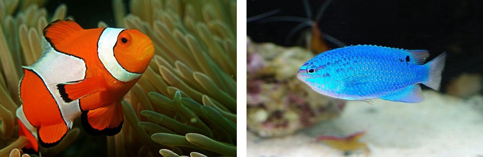
The dataset consists of pictures of clown fish and blue damsels. Within the training set there are 10 of each type of fish. Within the validation set there are 11 clown fish and 10 blue damsels. I typically include about 20% of the items in the validation set, but here I have 50% since this is such a small dataset.
The model I trained was Resnet-34. I won’t be going over the details of this model (maybe I will in a future post), but it is a state of the art convolutional neural network. We can take advantage that Resent (along with many other convolutional neural networks) has already been trained on the famous ImageNet dataset. ImageNet consists of a large dataset of over a million pictures that are from1000 categories. These categories range from animals to plants to inanimate objects. Even though models trained on ImageNet are trained to distinguish between these 1000 categories, it turns out that the trained layers are generalizable to other datasets. Researchers have visualized convolutional filters from models trained on ImageNet (see figure below) and filters from early layers detect low level visual features, such as edges, and it’s not until later layers that the filters pick up on features more specific to the trained dataset. What this means is that depending on the dataset, it may be the case that the pretrained filters may be applied to the dataset you are working with. Since we are training a classifier to distinguish between two types of fish and ImageNet contains fish, it may be very easy to use a pretrained model.
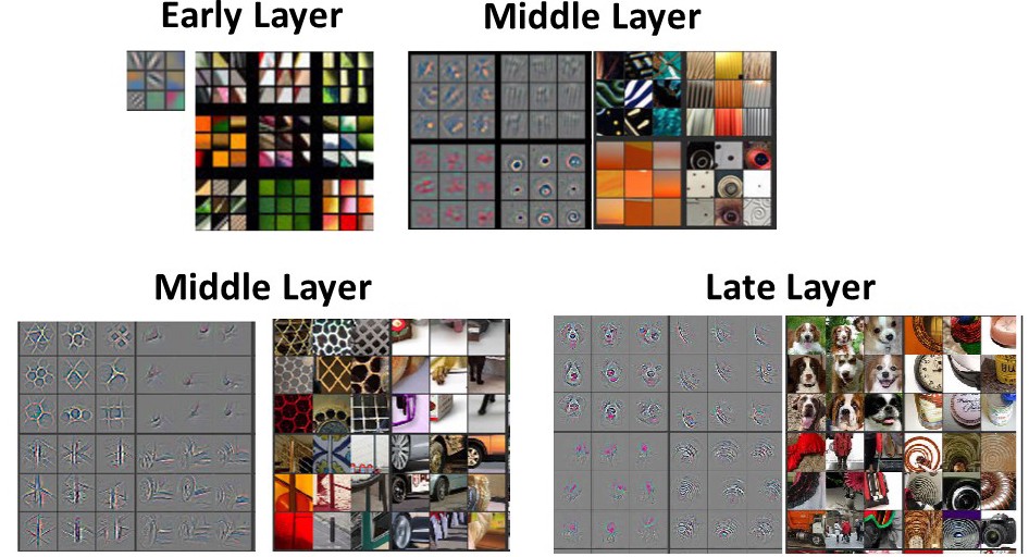
Image source: https://arxiv.org/abs/1311.2901
Training the Model
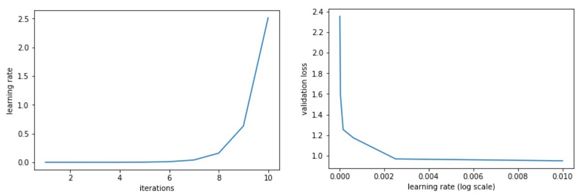
So lets start training the model! Again we are using a pretrained model. We will pop off the last layer (which distinguishes between the 1000 ImageNet categories) and add a new layer that distinguishes between clown fish and blue damsels. To start off, we are only going to train the last layer. Before we can start training, we need to choose the learning rate, which has traditionally been viewed as difficult to choose. A way to get around this is to use cyclical learning. With this approach the learning rate is varied and the change in loss is examined. We start off with a very low learning rate and gradually increase the learning rate. The figure below demonstrates this approach. The left figures shows that as the number of iterations increases, so does the learning rate. The right figure is how we choose the learning rate and shows the validation loss as a function of learning rate. Typically we choose the highest learning rate where the loss is still decreasing but hasn’t plateaued yet. Since this is such a small dataset, it is not completely obvious what learning rate we should choose, but it is usually more obvious with larger datasets that contain more iterations. Here, I chose a learning rate of 1e-2.
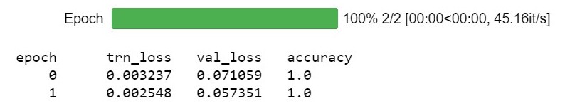
We are now ready to start training! As can be seen below (see the code for the full number of epochs ran), we have successfully trained our classifier with 100% accuracy to discriminate between clown fish and blue damsels! Not too difficult, right?
Improving the Model
Here we achieved 100% accuracy so we may not need to further improve the model, but with the vast majority of datasets, it takes a lot more work to achieve high accuracy. So here are a few techniques that I often use when training a convolutional neural network.
Data Augmentation
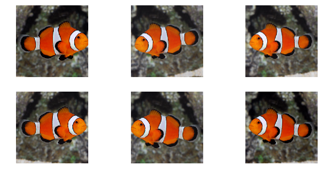
One way to improve a computer vision model is through data augmentation. Data augmentation slightly changes our images during each epoch. In a way this is like adding more data to a training set without collecting additional data, which sometimes is difficult or even impossible. This is a very powerful method and in my experience almost always improves classifier accuracy. Below is an example of the changes data augmentation may make to an image.
Differential Learning Rates
In the previous example, all we were doing was training the last layer and this worked fine for this example dataset, but a powerful approach is to train all of the layers but with different learning rates. Remember that our pretrained model comes from ImageNet. As discussed above, previous work has determined that filters from early layers detect low-level visual features, such as edges, and as we go deeper and deeper into the network, the filters start to pick up on higher-order visual features. So it is almost always likely the case that it will not be necessary to train earlier layers as much as later layers that are more specific to the trained dataset. How much we train each layer also depends on how similar it is to the trained dataset. In this example, we are training pictures of fish, which are also contained within ImageNet, so we are not going to want to change the earlier layers as much (or maybe even at all!) as the later layers.
Stochastic Gradient Descent with Restarts
My next tip is to use something called stochastic gradient descent with restarts (SGDR). SGDR is a variant of learning rate annealing, in which the learning rate is gradually decreased as training progresses. The theory is that as we get closer to the minimum, we need to starting using smaller learning rates so we do not miss the minimum. The problem is that we could get stuck in a minimum that is not very resilient and does not generalize well. So what we can do is jump back to a higher learning rate, start decreasing it again, and repeat this as much as you like. The idea behind this is visualized in figure below.
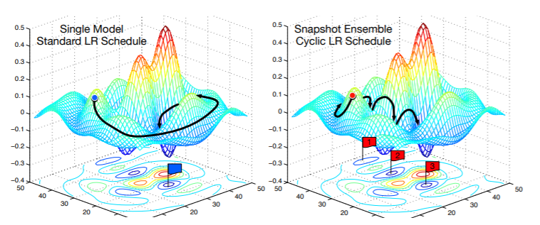
Image source: https://arxiv.org/abs/1704.00109
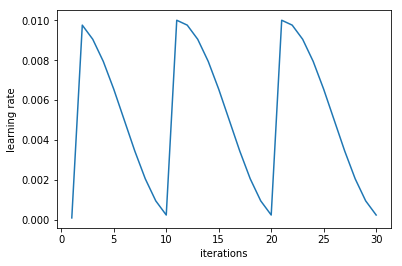
I used this technique on the example fish dataset, which can be seen in the figure below. The figure shows that the learning rate decreases as the number of iterations increases, but then the learning rate jumps back up (i.e, restarts).
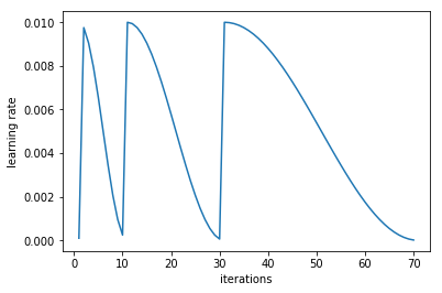
We can make this even better by varying how long it takes for the learning rate to decrease and, therefore, for a restart to occur. As training progresses, our model may be arriving at a more stable place in weight space that is closer to the minimum. Therefore, farther along in training, we may not want restarts to occur as frequently, so we can double (or multiply by whatever number you want) how long it takes a cycle to go from the highest to lowest learning rate. This can be visualized in the below figure.
Conclusions
As can be seen with this example classification problem, deep learning can be a very powerful tool to solve computer vision (among other) problems and works perfectly well even with small datasets. I hope this post will motivate machine learning practitioners that currently do not use deep learning to consider adding deep learning methods to their toolkit even if they do not have access to large computational resources. Deep learning has proven to be able to solve problems that were previously very difficult to solve and, therefore, I believe it is going to continue to revolutionize the field. Again, if you are interested in seeing the code and the example fish dataset, check out my GitHub.