Generative Adversarial Networks (GANs) for Beginners: Generating Images of Distracted Drivers

Generative adversarial networks (GANs) refers to a set of neural network models typically used to generate stimuli, such as pictures. The use of GANs challenges the dogma that computers are not capable of being creative. It is still early days in the utility of GANs, but it is a very exciting area of research. Here, I review the essential components of a GAN and demonstrate an example GAN I used to generate images of distracted drivers. Specifically, I will be reviewing a Wasserstein GAN. For reader’s more interested in the theory behind a Wasserstein GAN, I refer you to the linked paper. All of the code corresponding to this post can be found on my GitHub.
Let’s get started! A GAN consist of two types of neural networks: a generator and discriminator.
The Generator
The generator’s job is to take noise and create an image (e.g., a picture of a distracted driver).
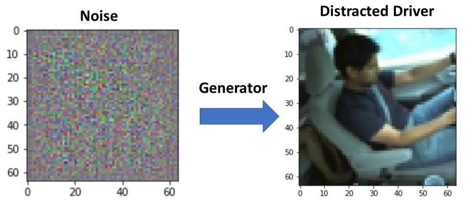
Generator
So how exactly does this work. Well we first start off with creating the noise, which consists of for each item in the mini-batch a vector of random normally-distributed numbers between 0 and 1 (in the case of the distracted driver example the length is 100); note, this is not actually a vector since it has four dimensions (batch size, 100, 1, 1).
We then have to go from a vector of numbers to a full image, which we do with the use of transposed convolutions. For readers that have previous computer vision experience, you are probably familiar with normal convolution layers that may downsample an image. For example, the figure below shows a convolution layer, with a 3x3 kernel, a stride of 1, and no padding. As can be seen, the size of the input is reduced from 4x4 to 2x2.
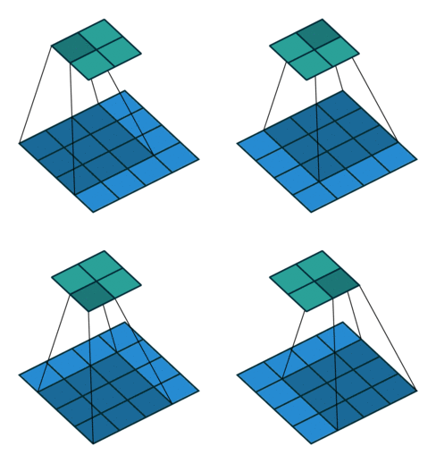
Convolution layer with a 3x3 kernel, stride of 1, and no zero padding. Image from the Convolution Arithmetic Tutorial.
There are also convolution layers with stride in which the filter “skips” cells. For example, below is a convolution layer with a 3x3 kernel, stride of 2, and no padding. As can be seen, the size of the input is reduced from 5x5 to 2x2.
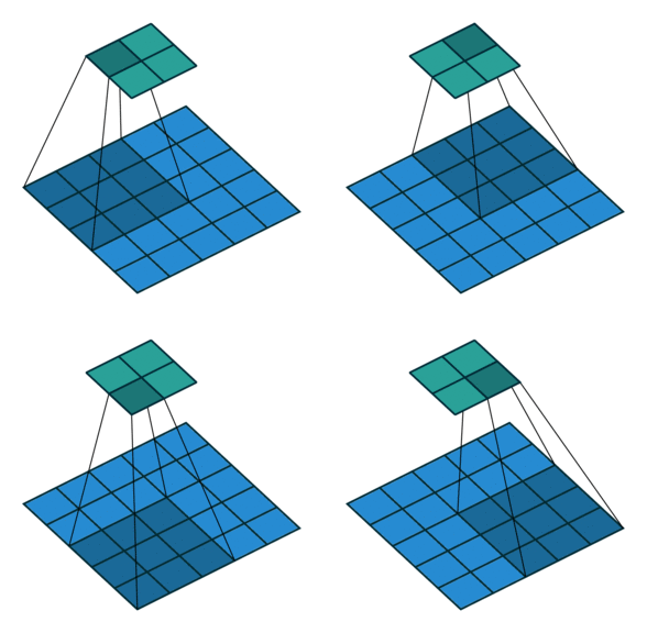
Convolution layer with a 3x3 kernel, stride of 2, and no zero padding. Image from the Convolution Arithmetic Tutorial.
With transposed convolutions, instead of the input being downsampled it is typically upsampled. For example, below is a transposed convolution layer with a 3x3 kernel, stride of 1, and no zero padding. As can be seen, the size of the input is increased from 2x2 to 4x4.
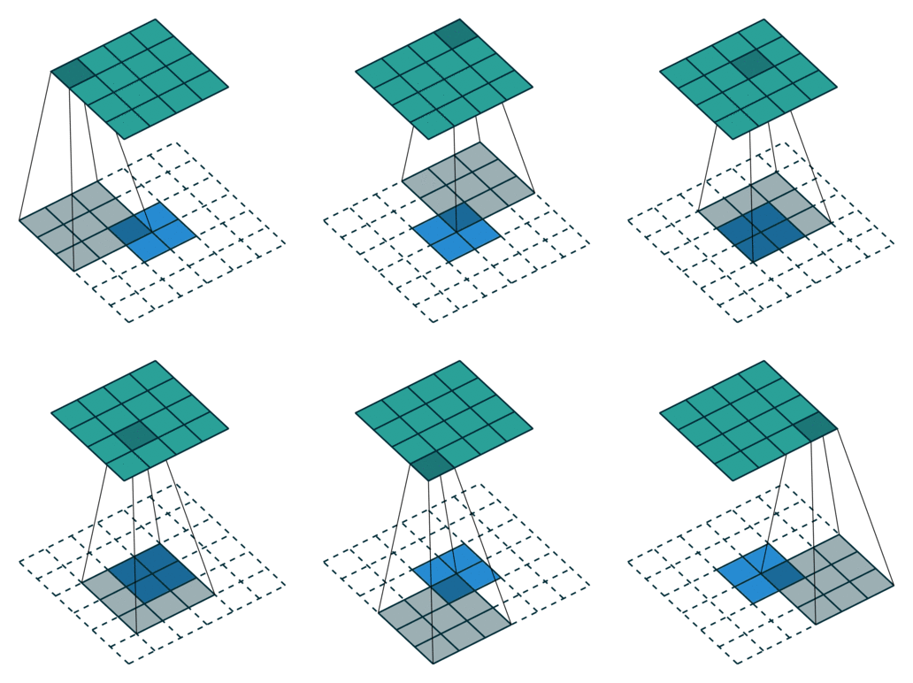
Transposed convolution layer with a 3x3 kernel, stride of 1, and no zero padding. Image from the Convolution Arithmetic Tutorial.
There are also transposed convolution layers with stride. For example, below is a transposed convolution layer with a 3x3 kernel, stride of 2, and no zero padding. As can be seen, the size of the input is increased from 2x2 to 5x5.
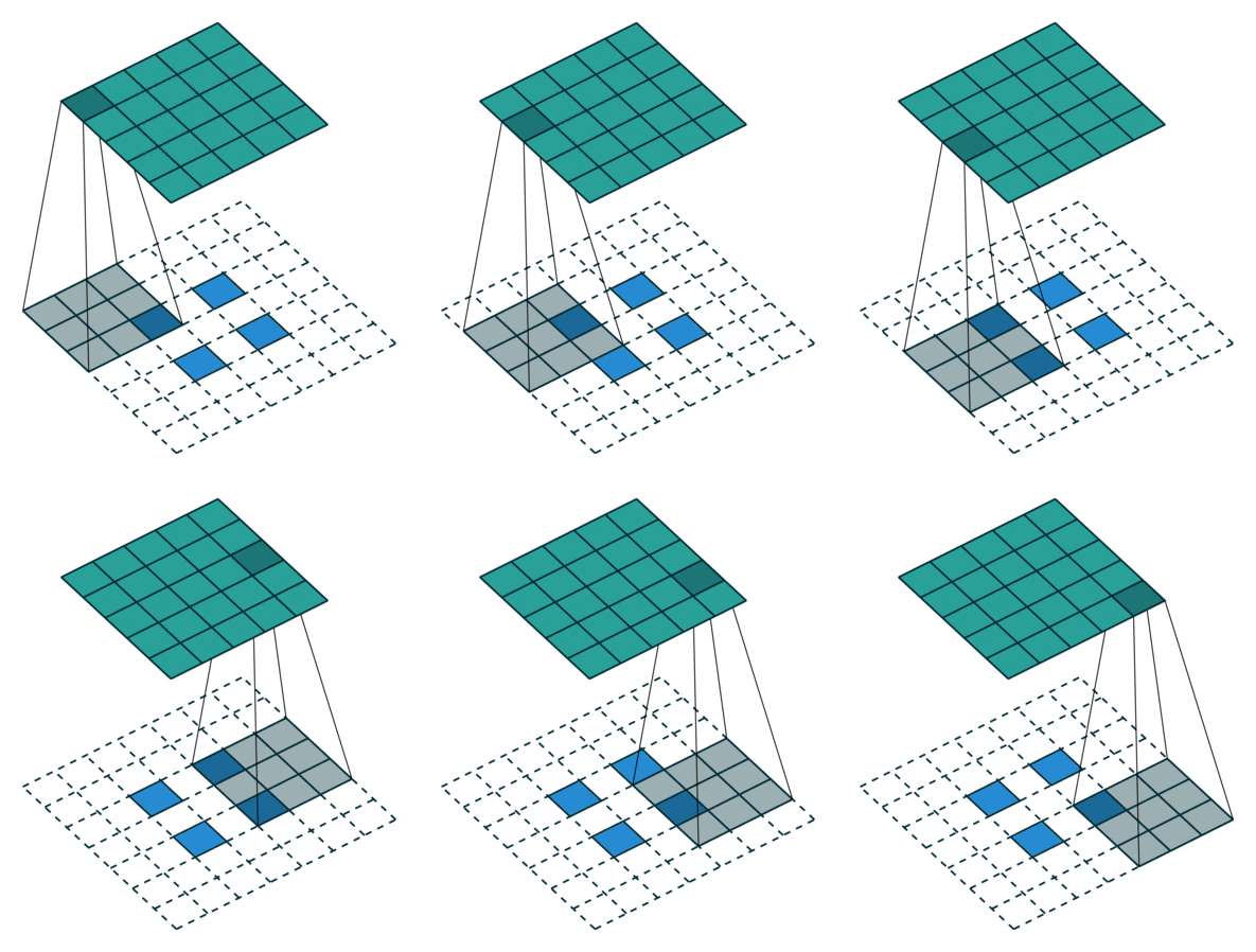
Transposed convolution layer with a 3x3 kernel, stride of 2, and no zero padding. Image from the Convolution Arithmetic Tutorial.
With the GAN generator, we essentially take the noise and upsample it until it until it is the size of an image. While doing this, we also reduce the number of filters. See the code on my GitHub for the exact details.
The Discriminator
The discriminator’s job is to take an image and try to decide if it is real or fake (i.e., discriminate between fake and real images). The model is actually quite simple, it essentially consists of using a whole bunch of standard convolution layers with stride to downsample the image eventually to the point where it is one value. This value is the loss. As described below in Training the Model, this loss is calculated for both the real and fake-generated images. While downsampling the “image,” we increase the number of filters. Again, see the code on my GitHub for the exact details.
Training the Model
Now that we have the generator and discriminator models, we can start training them! It turns out with GANs, it is important that our discriminator is really good at distinguishing between real and fake images. Therefore, we update the weights of the discriminator 5–100 times (see the code for details) for every time the generator weights are updated. Okay great, but exactly how do we train the discriminator? It’s actually quite easy. First, we take a mini-batch of our real images and put them through the discriminator. The output of the discriminator is the real loss. Then we put noise through our generator and put these fake images through the discriminator. This output of the discriminator is the fake loss. The discriminator loss is calculated by subtracting the fake loss from the real loss (real loss-fake loss). The weights are updated with respect to this loss. So as you can see, the generator is basically trying to trick the discriminator, hence the adversarial part of generative adversarial networks.
So how does the generator get good at tricking the discriminator? Well training the generator is actually quite simple. We just create some noise, put it through the generator, and put these fake-generated images through the discriminator. This output is the generator loss and is used to update the generator’s weights.
And that is all there is to training a GAN! Really not too complex. Now lets see a GAN in action.
Generating Images of Distracted Drivers
Here, I used the Kaggle State Farm Distracted Driver Detection dataset to train a GAN to generate images of distracted drivers (well I also included in training the non-distracted control drivers). The dataset essentially consists of a whole bunch of pictures of distracted drivers, such as drivers texting, putting on makeup, or talking to another driver. This dataset was originally released by State Farm as a Kaggle competition to train a classifier to detect how a driver is being distracted. If you remember a few years back, State Farm introduced the idea of having cameras in cars that would basically detect if a driver is being distracted and presumably adjust premiums based upon this information (I don’t actually know if that was their intention for detecting distracted drivers).
Lets start training! Just a small note, I originally downsampled the images to 64x64 pixels just so I could train the GAN faster, so the quality of these images is not as good as the original resolution. Below are 64 example generated images after one epoch. As you can see, they don’t look like really anything. Lets keep training.
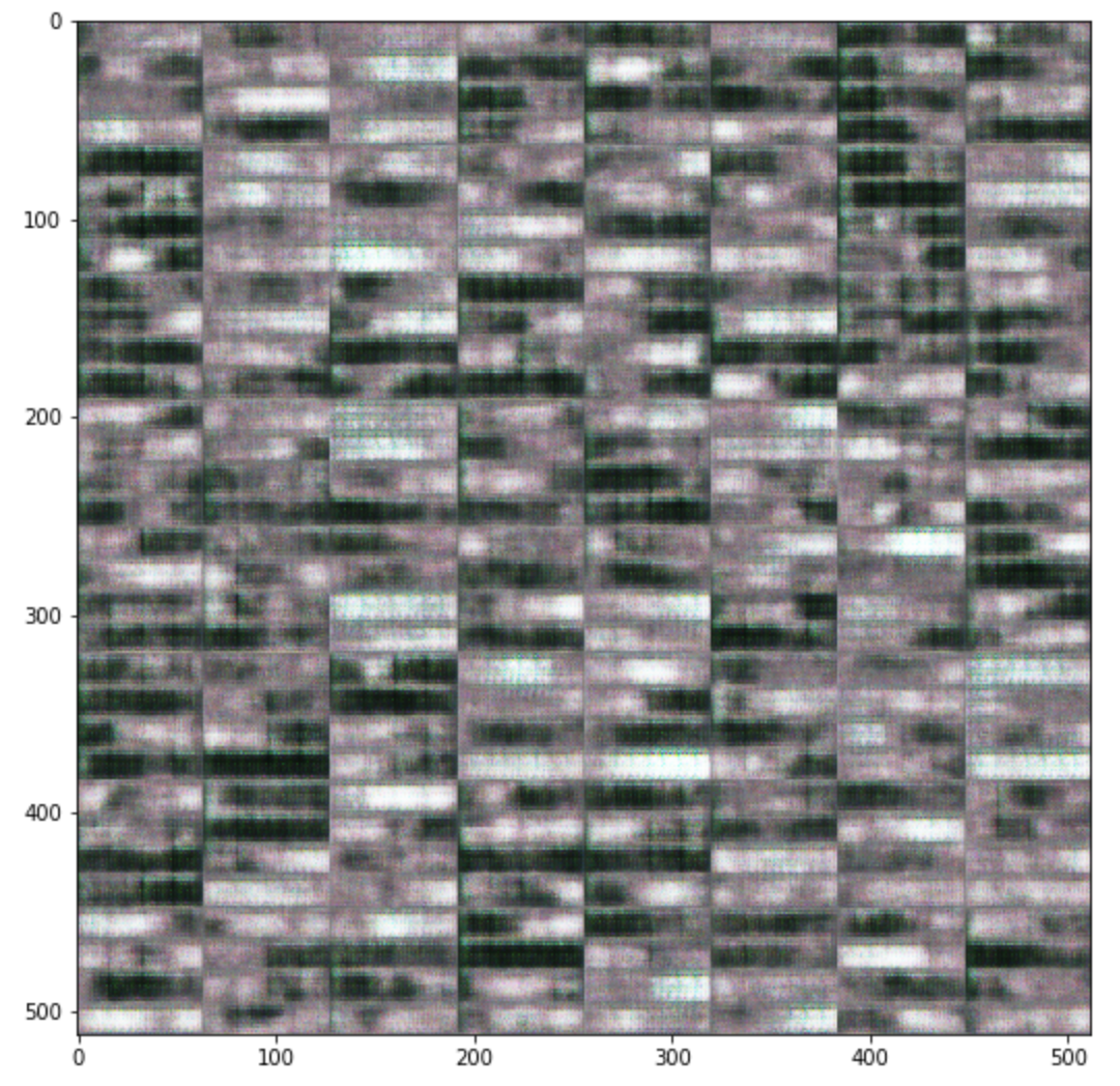
After 1 epoch
Now we can see below after 20 epochs, it does look like it is creating pictures of drivers in cars!
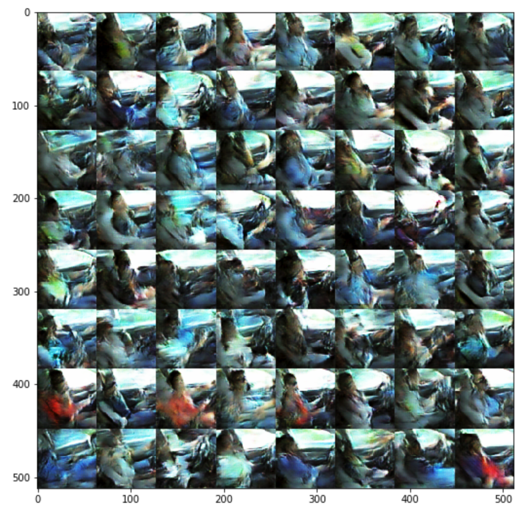
After 20 more epochs
After training for a little while, we get some pretty reasonable pictures. Take a look at two pictures below you can see an example generated distracted driver. It looks like this person is on his cell phone (cool!).
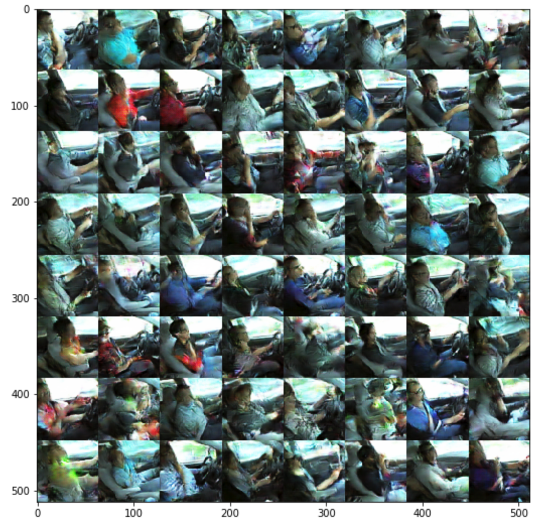
After training for a little while
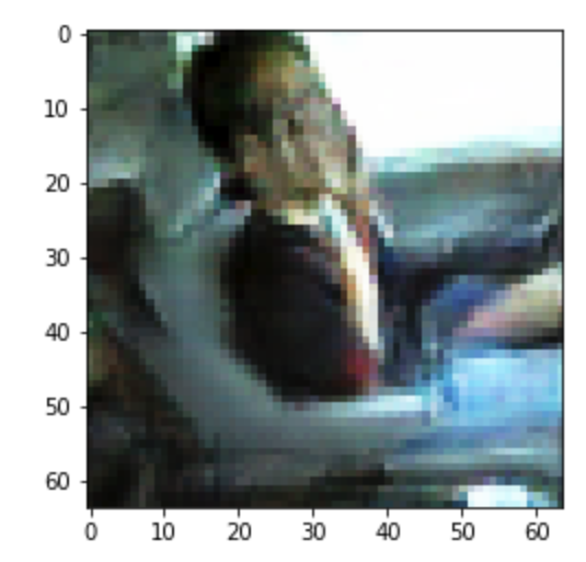
Generated distracted driver
Great! Are these images perfect, no, but for a very little amount of effort they are not too bad (at least in my opinion!). I find it truly amazing that a neural network is able to learn how to generate images. GANs are a really exciting area of research that are starting to break the assumption that computers are not capable of being creative. There have been many other recent breakthroughs in GANs (e.g., CycleGANs) that are even more interesting that I will likely write about in the future. Again, check out the code for this blog post on my GitHub and be on the lookout for future posts on GANs and other machine learning topics!