CycleGANs to Create Computer-Generated Art
An explanation of CycleGANs and demonstration of computer-generated art
CycleGANs refer to a subset of GANs which are capable of taking an image and generating a new image reflecting some type of transformation. The cool part of CycleGANs is you do not need paired images. This is really useful for scenarios where you may not have paired images. For example, if you want to convert pictures of zebras into pictures of horses. This kind of data would probably be impossible to collect, unless I guess if you painted zebras and horses… With enough creativity, they also turn out to be useful for creating computer-generated art that actually looks quite good!
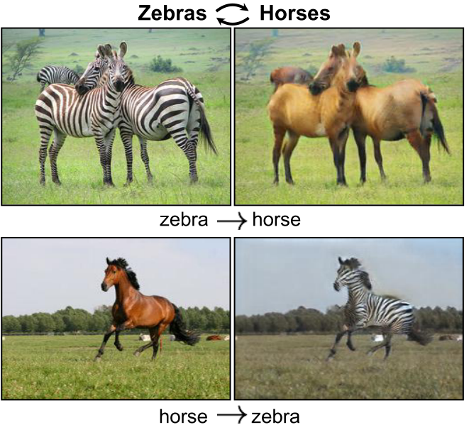
This figure is taken from the original CycleGAN paper.
Here, I will give an overview on exactly how CycleGANs work. This post does assume that you have at least some familiarity with GANs. So if you are not familiar with GANs, check out my blog post “Generative Adversarial Networks (GANs) for Beginners: Generating Images of Distracted Drivers.”
For this post, I use an example CycleGAN that was trained to convert pictures of forests into abstract paintings of forests. My code used to generate these images can be found on my GitHub.
The Dataset
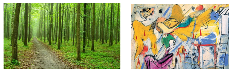
Here, the dataset consisted of forest images and abstract paintings. I scraped these images from Google Images using the keywords “forest” and “famous abstract paintings.” To do this I used the Python package Google Images Download. A couple examples are below.
The Model
When training a CycleGAN there are four neural networks that need to be trained:
-
A generator that generates pictures of abstract paintings (abstract painting generator).
-
A generator that generates pictures of forests (forest image generator).
-
A discriminator that can tell the difference between real and fake abstract paintings (abstract painting discriminator).
-
A discriminator that can tell the difference between real and fake pictures of forests (forest image discriminator).
If you are already familiar with GANs, you’ll see that there really isn’t anything new here. The novel aspect is in how these networks are trained.
Model Training
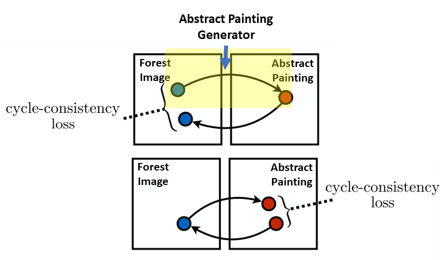
Before going into the details, let me give a high-level overview on how CycleGANs are trained. First, we take a forest image, use the abstract painting generator to create a fake abstract painting, and then we take the fake abstract painting and use the forest image generator to recreate the original forest image. We also go in the other direction where we take an abstract painting, use the forest image generator to create a fake forest image, and then we take the fake forest image and use the abstract painting generator to recreate the original abstract painting. This ingenious idea of the cycle is the novel contribution of CycleGANs and is shown in the diagram below. Something to note is that the same generator is used to generate fake abstract paintings and the reconstruction of abstraction paintings, and the same generator is also used to generate fake forest images and the reconstruction of forest images.
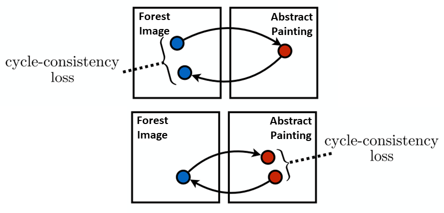
CycleGAN training. This figure is adapted from the original CycleGAN paper.
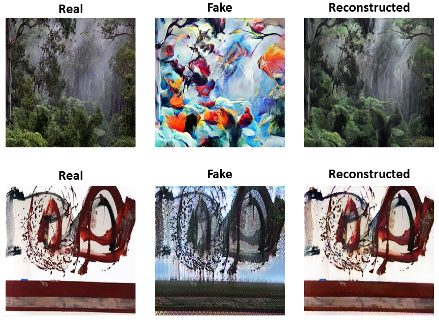
Below you can see how this actually looks with our CycleGAN. You can see the real images, being generated into fake ones, and then being reconstructed back into the real ones. You may notice, especially with the abstract painting, that the structures of the objects do not drastically change. This is a common observation with CycleGANs and is likely because of the recreation step. It may be too much for a CycleGAN to drastically change an image and then go back to its original version.
Okay now lets get into the details! When training the model, there are basically two steps: train the generators and then the discriminators.
1. Train the generators
Just like with any neural network, we need to calculate a loss (in this case for the generators) and use stochastic gradient descent with backpropagation (i.e., the chain rule) to calculate the gradients and update the weights with respect to these gradients. But how do we calculate the generator loss? This loss actually consists of a few different components.
First, we calculate the GAN loss for the abstract painting generator (in the “cycle” we are in the yellow shaded portion of the figure below). This is done by taking a real forest image and putting it through the abstract painting generator to generate a fake abstract painting. The fake abstract painting is then put through the the abstract painting discriminator. We can think of the output of the discriminator as being the probability that the picture is a real abstract painting. The output of the discriminator is then evaluated with binary cross-entropy loss. This is the abstract paining GAN loss.
GAN loss for abstract painting generator
Second, we calculate the GAN loss for the forest image generator (in the cycle we are in the yellow shaded portion of the figure below). This is done by taking a real abstract painting and putting it through the forest image generator to generate a fake forest image. The fake forest image is then put through the the forest image discriminator. We can think of the output of the discriminator as being the probability that the picture is a real forest image. The output of the discriminator is then evaluated with binary cross-entropy loss. This is the forest image GAN loss.
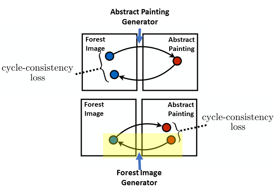
GAN loss for forest image generator
Okay great now we have a fake abstract painting and a fake forest image. As explained above in the high-level overview, we now have to take those fake images and reconstruct them back to the corresponding real images. So, third, we take the fake abstract painting and put it through the forest image generator to generate the reconstructed-original real forest image (in the cycle we are in the yellow shaded portion of the figure below). We evaluate this reconstructed forest image against the real forest image with L1 loss (Note, here, the L1 loss is typically multiplied by some constant so it is on the same scale as the other calculated losses). This is the forest image cycle-consistency loss.

Lastly, we take the fake forest image and put it through the abstract painting generator to generate the reconstructed abstract painting (in the cycle we are in the yellow shaded portion of the figure below). We evaluate this reconstructed abstract painting against the real abstract painting with L1 loss (Note, here, the L1 loss is typically multiplied by some constant so it is on the same scale as the other calculated losses). This is the abstract painting cycle-consistency loss.

Now we are almost ready to calculated the generator loss (yes, all of this work was for one number). There is one more loss we need to calculate, which is the identity mapping. The identity mapping loss is calculated because, as can be seen in the figure below, this step has been shown to preserve the colors of the original image. First, we put the real forest image through the forest image generator and calculate the L1 loss for the real forest image and the generated forest image. This is the forest image identity mapping loss (Note, this loss is also multiplied by constants). Second, we do the same thing for the abstract paintings, where we put the real abstract paining through the abstract painting generator. This is the abstract painting identity mapping loss.
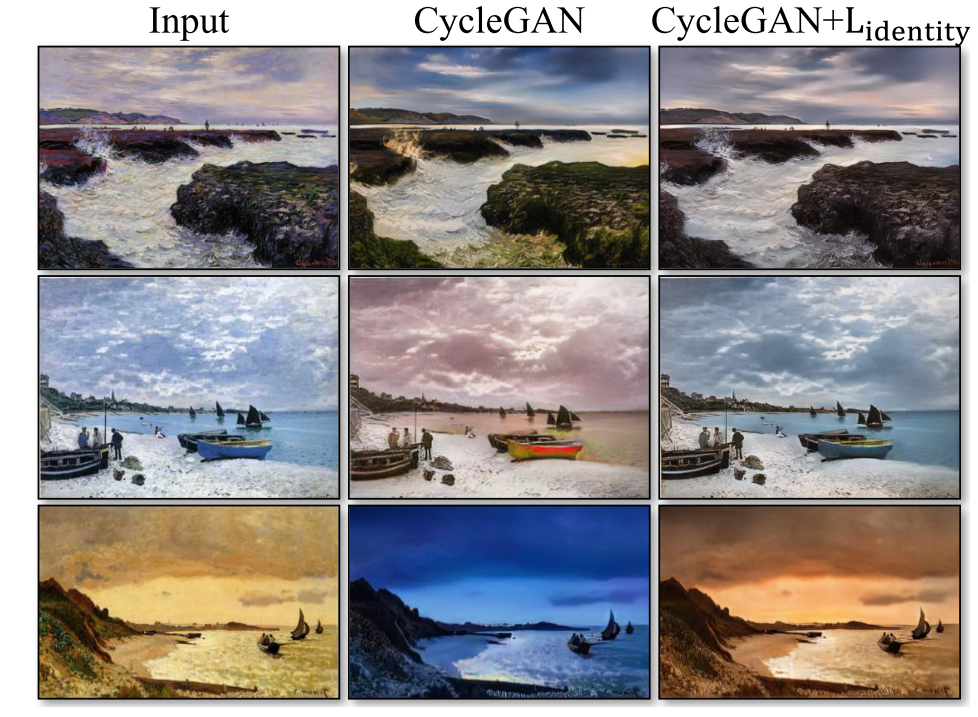
Figure 9 from the CycleGAN paper.
We are finally ready to calculate the generator loss, which are all of the loss components added up:
Generator Loss = abstract paining GAN loss + forest image GAN loss + forest image cycle-consistency loss + abstract painting cycle-consistency loss + forest image identity mapping loss + abstract painting identity mapping loss
The weights of the generators are then updated with respect to this loss!
2. Train the discriminators
Now that we have updated the weights of the generators, next we need to train the discriminators.
First, we update the weights of the abstract painting discriminator. We put a real abstract painting through the abstract painting discriminator and take this output and evaluate it with binary cross-entropy loss. Then, we take the previously generated fake abstract painting, put it through the abstract painting discriminator, and also evaluate it with binary cross-entropy loss. We then take the average of these two losses. This is the abstract painting discriminator loss. The weights of the abstract painting discriminator are updated with respect to this loss.
Second, we update the weights of the forest image discriminator. We put a real forest image through the forest image discriminator and take this output and evaluate it with binary cross-entropy loss. Then, we take the previous generated fake forest image, put it through the forest image discriminator, and also evaluate it with binary cross-entropy loss. We then take the average of these two losses. This is the forest image discriminator loss. The weights of the forest image discriminator are updated with respect to this loss.
The Architecture
So far I have mentioned that these generators and discriminators exist, but I have yet to say the exact architecture of these neural networks. Well there are, of course, a number of options for the architecture of these networks, but here I will briefly mention the architectures used to generate abstract paintings of forests. The details of these architectures may be viewed in the code. The generators come from an architecture previously used for style-transfer and super-resolution (see Johnson et al.). The network architecture basically consists of a bunch of ResNet blocks that downsample the grid size, keep the grid size constant, and then upsample the grid size. See the figure below for a diagram of the architecture.
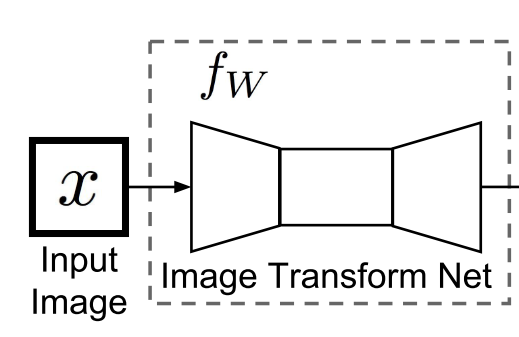
Generator architecture from Johnson et al.
For the discriminators, we used a PatchGAN, which basically tries to classify if each N x N patch (here, 70 x 70) of an image is real or fake. See the code and this paper for more details of the PatchGAN.
Computer-Generated Forest Images
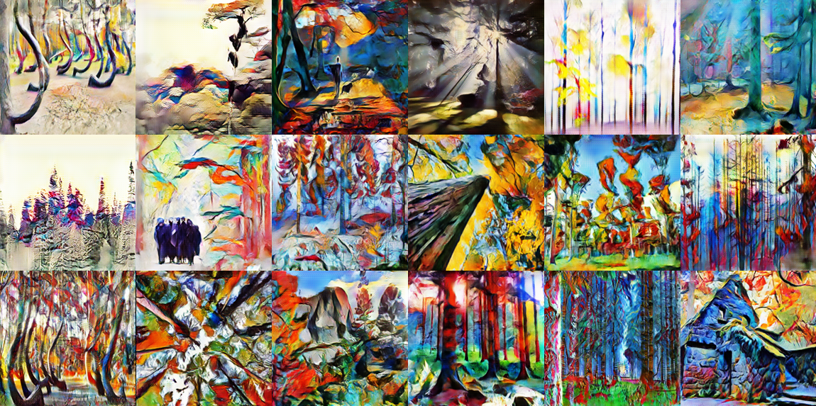
After training for awhile, lets see how our computer-generated abstract forest images look! Below are a few examples, but you can view all of them on my GitHub.
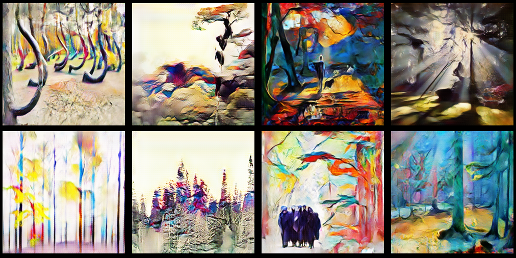
Not too bad! I created these images for an AI Art Competition at Duke University and I ended up winning first place — click here for more information.
Conclusions
As you can see above, it does indeed appear that computers can generate art thanks to CycleGANs in this case. Again, the really cool part of CycleGANs is that you don’t need paired images in the dataset. It is quite amazing that this is possible! I will be curious to see if unpaired machine learning is possible in other fields, such as natural language processing (maybe this already exists!).
***Update on 1/26/2020***: I forgot to post this earlier, but the art presented here won first place in an AI art competition at Duke University. Check out an article describing this competition!