Machine Learning Algorithms are Not Black Boxes
A Guide to Interpreting Neural Networks

Data science is a very new field with few standards set in stone. This makes it an exciting field to work in because it is up to current data scientists to create and set these standards. However, because data science is such a new field, there is a lot of misinformation out there. The #1 piece of misinformation I frequently hear is that machine learning algorithms are black boxes. I strongly disagree with this statement. I believe almost any machine learning is highly interpretable. Individuals saying that machine learning algorithms are black boxes also say they typically use linear models because they are more interpretable. I also strongly disagree with this statement and believe that many machine learning algorithms (e.g., neural networks, random forests) are more interpretable than linear models. The goal of this blog post is to discuss machine learning algorithm interpretability and present methods that can be used to interpret these algorithms.
Why you should care about model interpretability
Before going into the nitty-gritty details, lets discuss why you should care about model interpretability. Data science is different from many other sciences because most data scientists work in industry. This means that most data scientists use machine learning to solve business problems. This is probably the reason why the field is not as theory-based but rather more empirical-based — for the most part, data scientists don’t care as much about how theoretically elegant an algorithm is but rather does it work well or not. Model interpretability is often critical for solving business problems. Many in the field believe that machine learning is only used to automate processes. This is a use of machine learning, but there are many cases where I train a machine learning model not because I want to automate a process but rather I want to interpret it. In a business setting, you may want to know what are the most important features for a prediction and can I somehow manipulate or use those features to solve a problem of interest. For example, lets say you train a model that takes number of features and predicts if a customer will discontinue using your product or not (a customer retention problem). The process of automatically detecting if a customer is going to discontinue using your product is completely useless if you are not able to actually retain the customer (i.e., change the customer’s behavior). Therefore, identifying the customers at high-risk of discontinuation is just the first step. The next and most important step is identifying what should be done to change these customers’ behavior. This is where model interpretability comes in. We may want to examine what are the most important features for customer retention prediction. And out of those important features, determine the features that we can actually manipulate to prevent the customer from discontinuing. Machine learning is extremely well-suited for providing a data-driven solution to this problem. This part of the process requires some creativity and I encourage all readers to read Designing Great Data Products that discusses this issue in more depth.
Why linear models are actually difficult to interpret
Okay so we have discussed why model interpretability is so important, but you may still be thinking that since linear model is not as complex it is is better-suited for interpretation. I do not believe this is the case and here is why. First, properly fitting a linear model is very difficult. This is because linear models (linear regression/classification) have very constraining statistical assumptions (e.g., normality, non-collinear). With “real world” data, it is very rarely the case that data follows these statistical assumptions. The data could be pre-processed/transformed in an attempt to meet these statistical assumptions, but even when this is done, it is very often the case the data still does not meet all of these assumptions.
Second, interpreting beta-coefficients is typically flawed. Often when individuals are interpreting a linear model, they want to examine the feature that is most important in the model. This is done by after training the model, examining the beta-coefficients and examining the magnitude of these coefficients. However, this approach is often flawed. For beta-coefficients to be actually interpretable, the model would have to be constructed perfectly, meaning every main effect and interaction would have to modeled perfectly. But in almost all cases, it is impossible to know what main effects and interactions need to be modeled, so the beta-coeffients are basically useless. By the way, this is all assuming the relation between features and the dependent variable are linear, which is very rarely the case.
Why complex machine learning algorithms are easier to interpret
I hope by now I have convinced you that interpreting a linear model is not as easy as most people think. Now, you many be wondering why I think machine learning algorithms are easier to interpret. First, most machine learning algorithms have few statistical assumptions. This is the case for machine learning algorithms I use 99% of the time, which are ensemble-based algorithms (e.g., random forest) or neural networks. Therefore, these methods are able to handle “real world” data. Second, many of these algorithms are capable of learning complex interactions. Random forests and neural networks often contain many parameters. Individuals with a traditional statistics background often do not like using models with many parameters. They often fear these models will overfit to the training data. However, with the use of regularization, overfitting can often be avoided. Also, typically “real world” data is extremely complex and having many parameters is often necessary to sufficiently model the data. I would also like to point out to readers that checking if a model overfits is an empirical question. Experienced machine learning practitioners are able to recognize if a model is underfitting or overfitting and you can check (and should always check!) if your model is overfitting. In sum, machine learning algorithms are easier to interpret because they often can model your data more accurately.
How can you interpret a machine learning algorithm
Okay lets finally talk about how you can interpret machine learning algorithms. Here, I am going to discuss interpreting neural networks for tabular data (so data you typically find in a spreadsheet). You may be thinking why would you use a neural network with tabular data rather than some other algorithm like a random forest. Well, I do often use random forests, but recently I have come to find that neural networks many times outperform random forests (even when working with small datasets!). From my own experience, this seems to be the case when working with categorical variables. I believe this is because I use entity embeddings with my neural networks. Entity embeddings are out of the scope of this article, but if you are not using them, you should consider using them because they have helped me a lot. I refer readers interested in learning more about entity embedding to An Introduction to Deep Learning for Tabular Data.
All of the methods I show here were inspired by methods that are used with other machine learning algorithms besides neural networks (e.g., random forests). So this means these methods can be adapted for any machine learning algorithm. Also, all of the methods below are assuming that you have already trained your model, so this is what you would do after the model has been trained.
Lets get into it. Unlike interpreting a linear model where you often look at the parameters, when interpreting a neural network, I use interrogation methods. I often will make some type of experimental manipulation to the data and see how this affects my model output. Here, I present three model interpretation methods: feature importance, partial dependence plots, and individual row interpreter. For all my examples, I am using a fake dataset (Fig. 1) where I am trying to predict grocery store sales based often a few features (day of week, season, state, and year).
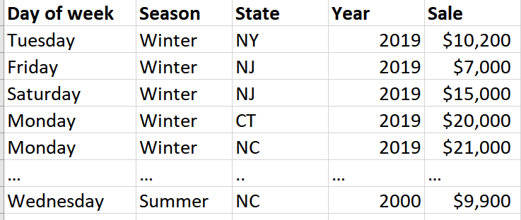
Fig. 1
Feature Importance
It is often the case that you want to know the most important features in terms of whatever your model is predicting. For example, in our grocery store example you many want to know what is the most important feature for predicting grocery store sales. You can do this by first, getting the loss of your final model (the baseline loss). Then, you are going to take one feature (so here lets say day of week as shown in Fig. 2), randomly permute (i.e., shuffle) those values (shown in Fig. 3), run your dataset through the trained model, and record your loss (the shuffle loss). Next, take of the absolute value of the difference between the baseline loss and shuffle loss. This is your feature importance. So if shuffling a value causes a large change in the loss, you can infer that this feature is really important for whatever your model is predicting.
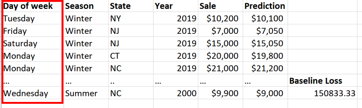
Fig. 2
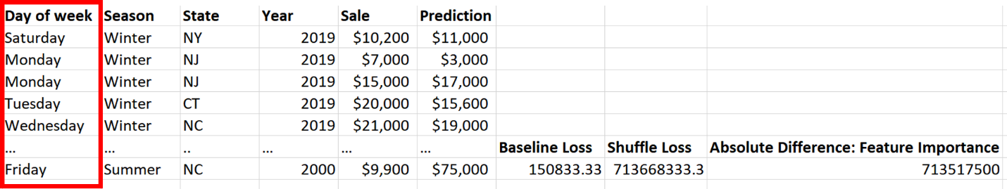
Fig. 3
You are going to repeat this procedure for every single feature. You then compare these feature importance values to determine the most important features. As you can probably see, feature importance is a relative measure, so that actual feature importance value itself does not matter too much, but rather it matters how it compares to all of the other features used in that specific model. Once you determine the most importance features, you may want to focus on these features when solving your business problem.
Partial Dependence Plots
A feature importance analysis tells us the most important features, but it does not tell how specific features are related to the dependent variable. The goal of partial dependence plots is to examine how a feature (or several features) is related your model dependent variable controlling for all other features in the model. So the really useful part of partial dependence plots is controlling for all the other features. The technique to create these plots is very clever, but simple. Lets say you have a model that is predicting sales at a grocery store and you want to see how the days of the week (Monday-Sunday) is related to sales. Again, your model has to already been trained. What we do is take one of the values from our feature of interest, so lets say Monday, and we change every row in the day of the week column in the dataset to Monday (Fig. 4). We then run that modified dataset through our model and get predictions. This is a very clever way of keeping everything else constant. So, in our example, in each row, the season, state and year are all kept exactly the same, but if day of the week in the row was not Monday, it is changed to Monday. This shows the specific effect Monday has on predicted sales. We then take the average prediction and store this value away.
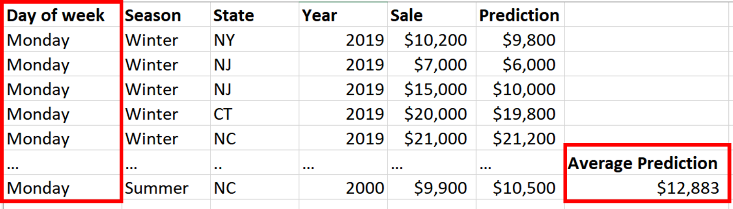
Fig. 4
We then do the same thing for Tuesday. Replace every row with Tuesday, run the modified dataset through our trained model, and calculate the average prediction (Fig. 5).
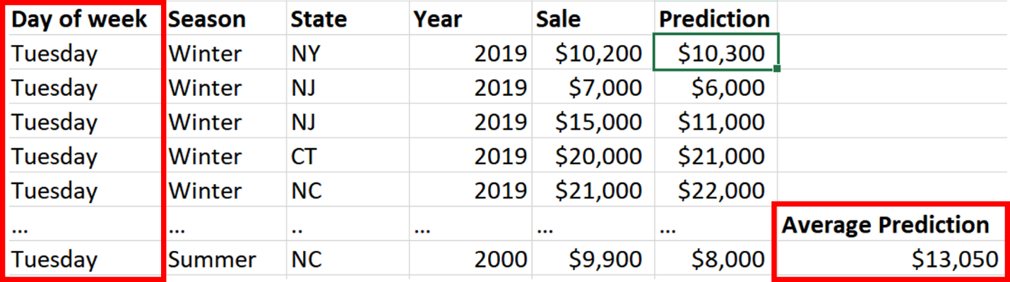
Fig. 5
We repeat this procedure for every day of the week and plot our results — this is a partial dependence plot (Fig. 6). The plot shows the relation between day of the week and the average sale prediction, controlling for all of the other features in our model. As you can see below (note: this data is not real), it appears that grocery sales are highest during Saturday and Sunday.
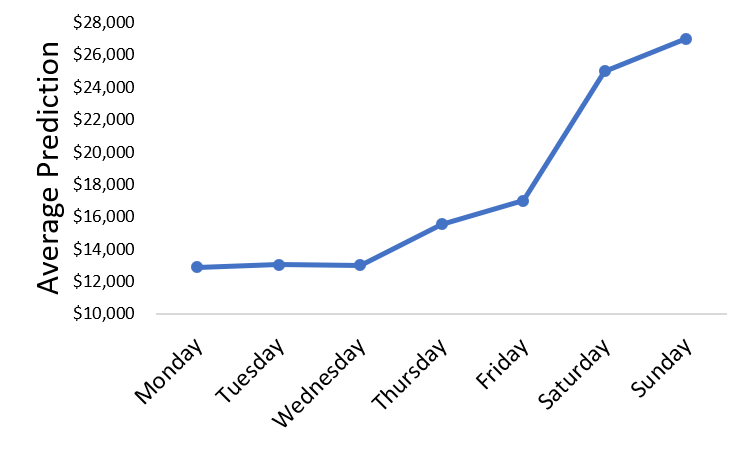
Fig. 6
I think this type of analysis is really useful. It would be difficult to examine this relation controlling for all of our other features without the use of a machine learning model. We are taking advantage of the complex interactions that a neural network has learned during model training. You may be thinking that this type of analysis is easily done with a linear model, but, again, to examine this type of relation all of the data would have to meet the statistical assumptions of linear models and we would have to model the data perfectly, which 99% of the time is impossible. With the use of neural networks, the model learns how to properly model the data.
Individual Row Interpreter
As you can see, feature importance analysis and partial dependence plots are examining group-averaged effects, but it is often the case that you may want to know why an individual observation was given a certain prediction. For example, in our grocery store sale example, you may want to know what features likely yielded a prediction for a specific row. The way we can do this is with individual row interpreter. I do have to admit that this method is somewhat more experimental than the feature importance analysis and partial dependence plots, but I have found that it does appear to work reasonably well.
This method was inspired and is very similar to tree interpreters that are used for interpreting random forests. There is a really good blog post about tree interpreters that I highly recommend readers check out — Interpreting random forests.
First, you need to choose the row that you want to interpret (Fig. 7). Now we are going to take the average prediction for the whole dataset. In this example, it is $13,700.
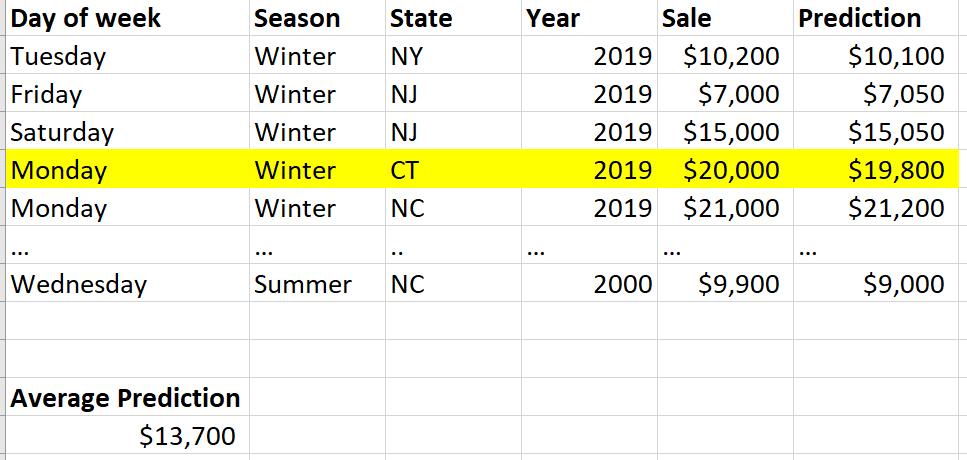
Fig. 7
Next, we are going to calculate the feature contribution for each feature. Lets start with day of the week. For this specific row, the day of week was Monday. So, we go through the dataset and find all of the rows that have Monday as the day of week (Fig. 8). Then for all of those rows, we take the average prediction. We then take the Monday rows average prediction and subtract from that the average prediction of the whole dataset, which yields $6,800. This is the feature contribution. We can infer that if the average prediction for a specific feature type (e.g., Monday) is really different from the average prediction of the whole dataset, then this feature is really important. Also, the direction of feature contribution is important. If the value is positive, it likely contributed to the prediction being higher than the average of the dataset, but if it is negative it likely contributed to the prediction being lower than the average of the dataset. As you can see, just like feature importance, this is going to be a relative measure.
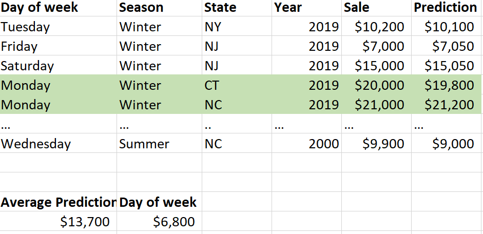
Fig. 8
Now let’s do this for our next feature, which is season. For the specific row we are interpreting, the season was winter. So we are going to find all of the rows where the season was winter, get the average prediction, and compare the winter average prediction to the average prediction of the whole dataset; here, the feature contribution for season was $940 (Fig. 9).
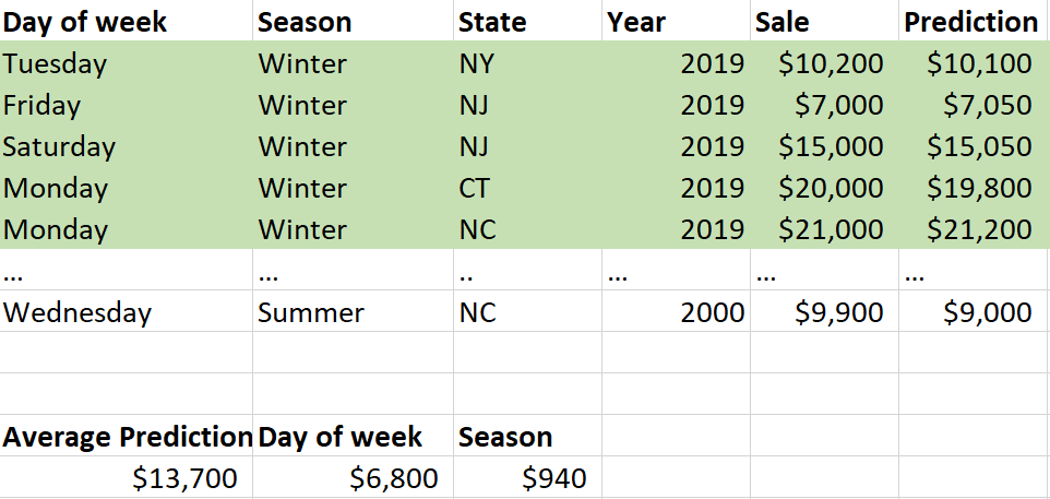
Fig. 9
We are going to repeat this procedure for all of the other features (Fig. 10). Now we can look and see the most important feature for this specific row. In this case it is day of week — also show in a plot (Fig. 11). In our example, all of the contributions were positive, but also keep in mind that contributions can be negative. If you have a mix of positive and negative contributions and you are struggling to find the most important feature (so maybe you don’t care about the direction of the change), you can, of course just take the absolute value of these contributions.
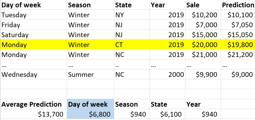
Fig. 10
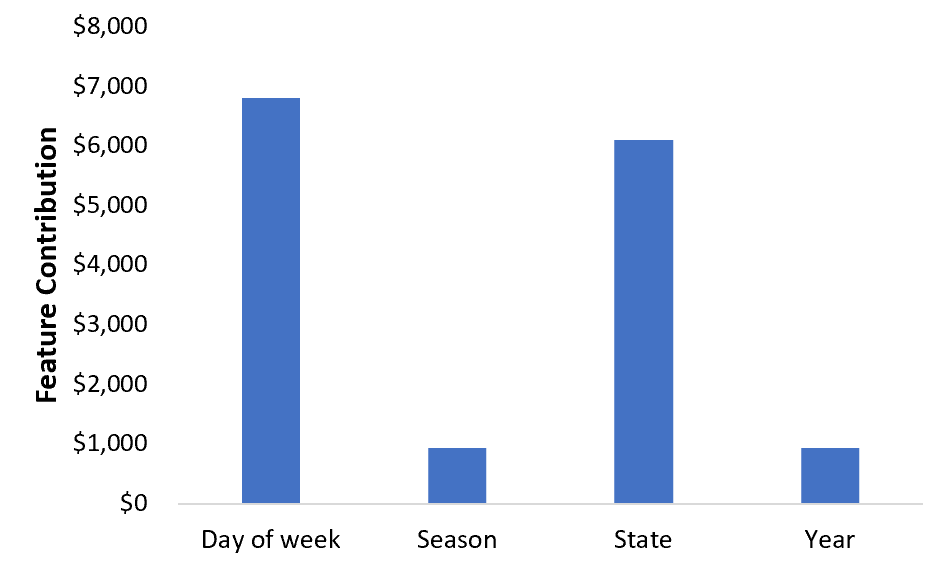
Fig. 11
In our example, all of our features were categorical variables, so you may be wondering what to do with continuous variables. This is again somewhat experimental, but for a continuous variable, I bag values into one of two different categories. The way I do this is by taking all of the values from the dataset of a specific feature and sort the unique values. Then, I find the value where I can split the dataset into two groups (so bagging values lower than or equal to the split point value and values higher than the split point value) where the difference in the average predictions is the largest (very similar to a decision tree!). When calculating feature contribution for this continuous variable, you can look at the value and see does it belong to the category that is less than or equal to the split point value or to the category that is greater than the split point value. Then, you calculate feature contribution normally.
Conclusions
As you can see from these methods, none of them are complex and I hope these inspire readers to develop other/better methods of interpreting machine learning algorithms. I hope I have convinced you not only that machine learning algorithms are highly interpretable, but they are extremely useful in solving business problems (or any type of problem). Many of the insights provided by machine learning interpretation often cannot be achieved with simple descriptive statistics.
Machine learning model interpretation is still in its infancy so feedback and new ideas would be greatly appreciated — either in the form of comments here or new blog posts! Have fun exploring your machine learning algorithms!