Time Series Anomaly Detection With “Real World” Data

Time series anomaly detection is a very hard problem, especially when working with “real world” data. To illustrate what I mean by “real world” data, let’s say you are working with multiple clients and each client is running a different longitudinal study. The clients want you to help them detect anomalies in their data while the study is running, so they can potentially fix these anomalies and improve data collection quality. You may already have some ideas how this can be a hard problem. First, unlike what you may see in a Kaggle competition, it may be the case that the data is not labeled (i.e., you do not actually know what is an anomaly and what is not), which is actually quite common! Perhaps the clients did not have the resources to create a labeled dataset. Second, in this case, where every client is running a different study, it is very likely that each client will have different features in their datasets, not allowing for a single model to be used for all of the clients. Third, longitudinal studies are often quite expensive to run and, therefore, each of the client’s datasets may be relatively small. Lastly, since each of these studies is still in progress, there may be a lot of “missing data.” In this case what I mean by missing data is that different subjects will be at different points in the study, where perhaps some will have only completed two visits whereas other may have completely finished the study.
So to briefly summarize, in this example, there is a lot working against us: we have (1) unlabeled data, (2) datasets with different features, (3) small datasets, and (4) datasets with a large amount of missing data. This may sound like a nightmare to many data scientists! But there are ways we can still find value in the data and detect anomalies. Here, I briefly present a method I have recently used which I have found to pick up on reasonable signals. Unfortunately, at the time being, I am not able to release details of this project, but I hope you also try out this method and let me know how it works.
The Method
I have recently become a big fan of the isolation forest. The isolation forest is an ensemble learning method and is a close cousin of the random forest. Similar to a random forest, an isolation forest uses decision trees, where you make decision splits in features. The biggest difference between a random forest and isolation forest is that in an isolation forest, the splits are random. What is typically done is the isolation forest chooses random features and makes random splits in features until all of the data points are isolated; this procedure is conducted several times using as many trees as you would like. We assume that if a data point requires many splits to isolate, then it is not anomalous (left panel in the figure below), but if a data point requires very few splits, then it is an anomaly (right panel in the figure below). The output of an isolation forest is an anomaly score, which indicates how anomalous a data point is considered. As you can probably tell from the description of this algorithm, it is an unsupervised anomaly detection method, which is necessary for us since we don’t have labeled data. This is quite a simple method, but it works reasonably well! Also, the isolation forest is included in scikit-learn so it is relatively easy to implement.
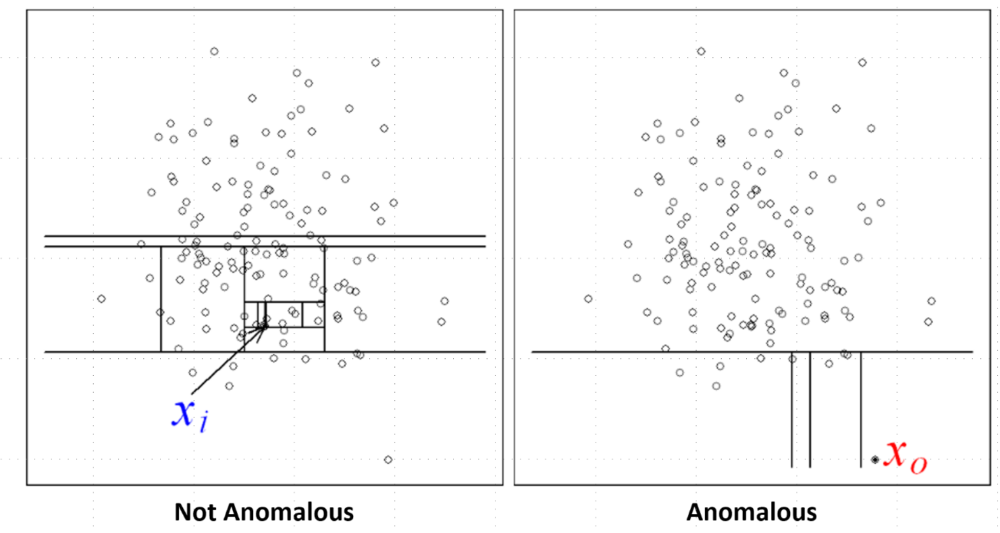
Figure from original isolation forest paper.
Okay, it sounds like the isolation forest has solved a lot of our problems, right? Nope! We still have this issue of “missing data.” Let’s go back to our longitudinal study that is currently still in progress and we have subjects at different points in the studies. As you may know, most machine learning algorithms cannot include missing data, so a common method to handle missing data is to impute missing values with the median (or create a new category for categorical data). This may work fine in many cases, but what about in our example where let’s say there are a lot of subjects that are still early on in the study. For these subjects, we can impute the missing values with the median for the visits they have not completed yet and run the isolation forest on our dataset. However, if you do this, you may notice that subjects that have completed very little visits never appear to be anomalous and that is simply because we are causing them to appear more normal by imputing the missing values with the median. This is not good! We want to detect anomalies that might be appearing in any subjects whether or not they are earlier in the study or have already completed the study.
So what can we do? Well, there is a relatively easy solution to this problem. We run separate isolation forests on subjects that completed each visit. For example, let’s say a study has five subjects. Subjects 1, 3, and 5 have completed six visits, whereas subjects 2 and 4 have only completed the first three visits. What we would do is run the isolation forest using data for all six visits for subjects 1, 3, and 5 and output the anomaly scores. Then for subjects 2 and 4, we only use data for the first three visits and also include data from the other subjects too (only data from the first three visits), but we just output the anomaly scores for subjects 2 and 4. This method greatly reduces the number of data points in which we need to impute missing values with the median and, therefore, allowing all data points to potentially be considered anomalous. Great!
Model Interpretation
If you’ve read my previous blog post, you know that I am passionate about model interpretation. Understanding the features driving a prediction are often critical for solving business problems. For example, going back to the longitudinal study example, if you find that a subject is anomalous, you will probably want to know why they are anomalous and try to resolve, if possible, whatever issue is causing them to be anomalous. So how can we interpret an isolation forest model? The approach is very similar to the feature importance analysis method I discussed in my previous blog post. First, we run the isolation forest as normal and output the anomaly scores — these are the baseline anomaly scores. Then we take a feature, shuffle its values, re-run the dataset through the isolation forest, and output the anomaly scores. We conduct this procedure for every feature in the dataset. Then, the anomaly scores for each shuffled feature are compared to the baseline scores. We can infer that if there was a large change in the anomaly scores, then this was an important feature in terms of detecting anomalies. This can even be examined at the level of individual subjects, where we can examine changes in anomaly scores from a single subject. Very simple and I have found gives a reasonable output!
Conclusions
Well, there you have it. I recognize this approach isn’t perfect and that there are many alternatives, but I wanted to share a method that I found works reasonably well. Feedback and alternative ideas are more than welcome!